STRUCTURAL MECHANICS AND ANALYSIS OF CONSTRUCTIONS   ISSN 0039-2383          №3  2019,  p.31-38

УДК 624.044

TO THE QUESTION OF DETERMINING THE BUCLING LENGTH OF RODS ELEMENTS OF FRAME SPACE SYSTEMS

E.I.Britvin, Ph.D

 

An efficient computational algorithm was constructed, which allows finding the buckling lengths of the rod elements of frame structures. A matrix of reaction from the side of the truncated part of the system is formed for each element and the problem of the eigenvalues of longitudinal bending equation of the rod is solved. When searching for eigenvalues, the stress state of the system is fixed. The solution is exact. High speed of algorithm is demonstrated.

Checking the local stability of the core elements is one of the most important checks necessary to ensure the reliable operation of building structures. Virtually no one analysis will complete without this verification. At the same time, each designer knows how much uncertainty this test conceals. The problem is that for its implementation for each rod, the designer must set the so-called "buckling length". As a rule, software systems are able to produce this parameter (buckling length is a byproduct of checking overall structural stability). But very often the calculated values are beyond reason. In particular, for lightly loaded rods, the program can produce huge quantities that do not fit into any natural idea of the nature of this test. A similar situation occurs if some weak rod “wormed” into the structure, losing stability much earlier than the whole structure (degenerate form of buckling). In this case, the program calculates the buckling parameters of all other rods, focusing on this found conservative critical value, giving out the complete absurdity. Practice shows that the buckling lengths calculated by the program can actually be used no more than for 5-10% of the core elements included in the structure. For other elements, the calculator should refer to various reference books and norms [3] - [6], which do not always cover all possible cases. Some authors propose semi-analytic solutions, highlighting a limited fragment of the structure adjacent to the tested rod element [1], [2]. Unfortunately, only a very experienced designer can understand this situation, understand when it is possible to use the data provided by the analysis, or should refer to the directories. Therefore, checking the local stability of the core elements often resembles cartomancy.

To overcome this problem, the authors in due time developed a special algorithm [7], which allows one to evaluate the operability of a structure without using the concept of “buckling rod length”. The reason for the premature (in comparison with Euler's theory) loss of stability of the rod elements is the presence in the rods of small, invisible to the eye, initial imperfections (in other words, small initial curvatures). Therefore, even with central compression of such a rod, a moment stress state arises in it. If with an load increase, the total stress from compression and bending in one of the fiber of the rod reaches the yield point, then irreversible changes occur in the body of the rod and the rod loses stability (loss of stability of the second kind). Based on the physical model of this phenomenon, a special finite element of the rod with an initial imperfection in the form of a parabola was developed. The limiting values of imperfection depths were normalized by the corresponding building norms. Given that the imperfection depth is a random variable, the algorithm performed a series of calculations according to the deformed scheme, randomly generating signs and values of the imperfection amplitudes. It was assumed that the depths of the imperfections are distributed according to the normal law in the interval [0, X], where X is the limiting value of the depth of the initial imperfection. The distribution center was taken at point X/2. Standard of distribution was taken equal to X/5 (value X/5 was chosen arbitrarily – the studies showed that the result vary little depended on the size of the standard). As a result, according to the formed samples, for each rod, the algorithm calculated the mathematical expectation and the standard of deviation of fiber stresses. Based on these data, by means of statistical processing for each rod, the ultimate fiber compressive stress was determined, which would not be guaranteed to be exceeded with a given probability. Comparing this stress with R_y, a conclusion was drawn about the bearing capacity of the rod. The algorithm was successfully implemented on the Selena software package [8].

Since our domestic building norms do not provide for this type of verification (note, in Eurocode 3 [5] there is a direct resolution of verification taking into account initial imperfections), despite the significant relief, users of the program still, in conclusion, had to corroborate the analysis with a standard verification of local stability of rod elements according to the building norms technique. Usually, the solution was as follows: at first, users selected the necessary sections based on the analysis according to the program (the program in a very visual form allows to identify all weak elements), and then, with a much lower risk to “miss the mark” in the choice of buckling lengths, a standard check was performed. But even in this situation, the need to set the estimated lengths, which most often, no one knows where to get, is associated with a large amount of manual work and significant psychological inconveniences.

The purpose of this work is to look into, if possible, what exactly is “buckling length” and, possibly, give recommendations for their determination. Physically, the buckling length of the rod is the distance between a pair of neighboring zeros on the diagram of the moments of the rod, subjected to longitudinal bending. By this, it is believed that an arbitrary rod is reduced, as it were, to a rod hinged at both ends, for which the solution of the problem of longitudinal bending is well known. Among experts, however, there is an opinion that the method for checking the buckling of core elements based on buckling lengths does not have a clear scientific justification. In fact, this is not entirely true. It can be shown that the test procedure for an arbitrary rod subjected to longitudinal bending can be performed according to the same formulas as the pin-ended rod. Unfortunately, the author was unable to find this evidence in the literature (although there is great suspicion that it still exists somewhere). Therefore, we present here this short conclusion, especially since its result is very important for our further presentation.

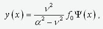
Figure 1 shows the rod with the initial imperfection specified by the function f(x). A longitudinal compressive force acts on the rod N. As a result of deformation, the rod acquires additional displacement y(x). Reactions of the truncated part of the structure are conditionally shown in bold dotted lines.

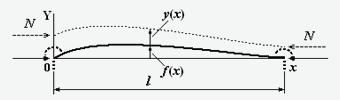
Fig.1

The equation of the longitudinal bending of the beam, with the initial imperfection f(x) has the form (Fig. 1)

Let the initial imperfection is described by an expression of the form

where f₀ – “depths” of imperfection, and Y(x) – some normalized function in a certain way. In the first approximation, we assume that the function Y(x) сcoincides with the solution of a homogeneous differential equation of the form (1) under the corresponding boundary conditions. That is Y(x) satisfies the equation

,

where a – is the eigenvalue of the boundary problem. The solution to this equation is an expression of the form

.

Without loss of generality, we normalize this expression so that the condition B²+C²=1. Obvious expression

,

is a solution of equation (1), where n²=N/EJ. This can be easily verified by substituting (5) in equation (1). Moreover, the solution y(x), by the definition of the function Y(x), will satisfy the given boundary conditions. That is, what is required.

Express the bending moment in the beam according to the formula . Given expression (4), we obtain

.

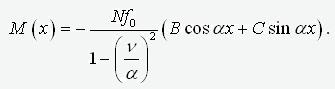
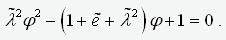
Since the buckling length of rod l_p– is the distance between the zeros of the moment diagram, immediately follows from expression (6) – al_p=p. And the extremum of this expression is reached at the point x₀, satisfying the condition cos(ax₀)=B и sin(ax₀)=C. As a result, we get

.

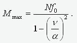Thus, the physical meaning of the “depth” f₀ – this is the amplitude of the roughness over the linear component. We calculate the fiber stress at the point where the moment reaches its maximum

.

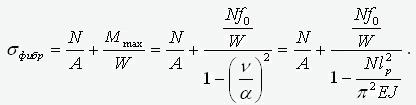where A, J and W – area, moment of inertia and moment of resistance of the section. We transform this expression as follows

.

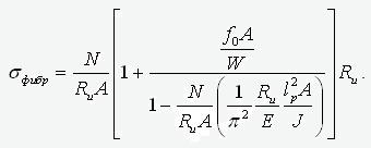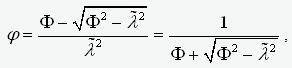
Considering that J/A=i² - is the radius of inertia of the section and l_p/i=l - flexibility of the rod, and also introducing the designations 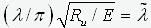- reduced flexibility, - reduced eccentricity and N/R_uA=j, we obtain

.

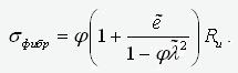
We now determine under what condition the fiber stress reaches the yield strength, i.e. . As a result, equation (7) takes the form

.

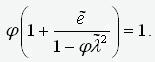Getting rid of the denominator in this expression, we arrive at the quadratic equation

.

His solution

,

where .

Thus, through a small generalization, we were able to show that formula (8), which is usually derived for a pi-ended rod, is applicable without change to the general case of fixing the ends of the rod. This conclusion, of course, cannot be considered as strict. Firstly, we limited ourselves to the form of imperfection, and the question of choosing the worst form remained open (although intuition suggests that there is a rational grain in our choice). Secondly, finding the maximum of the moment, we did not investigate the values at the boundary of the interval. But the choice of the extremum point as the maximum of expression (6) guarantees us that the maximum value of the moment on the segment [0,l] will be at least no more than the selected value.

This study has another drawback. Despite the fact that the roughness enters into equation (1) through the second derivative, and it seemed that this makes it possible to vary the linear terms in expression (4), the solution can be considered fair only if the shape of the initial roughness is strictly proportional to the natural mode of the rod stability loss. Because only in this case the solution (4), (5) will strictly satisfy the boundary conditions of the problem. On the other hand, by imperfection we are used to understand the deviation from the line connecting the attachment points of the rod. This means that at the beginning and end of the rod this function must be equal to zero, which is by no means always an indispensable attribute of the mode of stability loss. Thus, the “pressed” to the ends of the rod equivalent of expression (4) is the expression

,

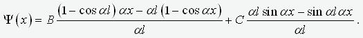
Figure 2 shows the diagrams of the moments of the cantilever rod, compressed by the same force equal to half the critical for various forms of the initial imperfection: a). in the form of buckling - ; b). parabola - 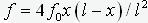; c). on the “pressed” form of buckling - . For all three cases, the normalizing coefficient was taken equal f₀=0.01. Rod parameters – l=2, EJ=1.

Fig.2

Dashed lines show the shape of the imperfection on an exaggerated scale. Diagrams of moments are defined by expression

where al=p/2, n²=N/EJ. Near the diagrams the maximum values of the moment are shown. As you can see, the greatest value of the moment turned out for option a. - imperfection proportional to the buckling mode. Note that exactly this form of imperfection that is embedded in the above conclusion, the final result of which is formula (8). In the framework of this study else several numerical experiments on the simple frames were performed. Due to limited space, we do not present these results. But in all cases, an imperfection proportional to the form of stability loss, ceteris paribus, gave the greatest maximum moment. This study, of course, cannot be considered as evidence that imperfection in the form of a buckling mode of the rod will always lead to the greatest moment. But one can make the assumption (praesumptio) that in most cases this will be exactly so (especially since when the force approaches a critical value, the shape of the deformation curve will inevitably tend to a buckling mode).

From the foregoing it follows - in order to determine the value of the longitudinal force in a separate rod, at which a stress equal to the yield strength arises in one of its fibers, it is necessary: 1) solve for this rod the problem of the eigenvalues of the equation (3); 2) using the formula l_p= p/a calculate the buckling length of the rod (a – eigenvalue); 3) from the buckling length l_p go to the flexibility l and, using formula (8), calculate the buckling coefficient j; 4) determine the desired ultimate value of the force N=jR_uA (more precisely, its lower boundary). The most difficult part in this list is, of course, to solve the boundary value problem for equation (3). The task become complicated by the fact that the conditions at the ends of the test rod are provided by reactions in the attachment points of the rod from the rest of the structure. In other words, we must be able to calculate the reaction matrix from unit displacements of bonds restrictions on a pair of nodes to which our core is attached. Moreover, in order to be able to vary the force value in the tested rod itself, we must first exclude this rod from the structure.

The standard procedure for finding the buckling lengths of the rod elements consists of two stages: first, the longitudinal forces in the rods from the given load combination are calculated, then a uniform factor for all the found forces is introduced and its critical value is found at which the system loses stability. Based on the found forces N_кр,i, corresponding to the critical state, the buckling lengths of the rods are calculated by the formula 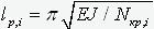. Obviously, this process is completely equivalent to the procedure described above, with the difference that when solving the problem of eigenvalues of equation (3), along with the changing force in the test rod, the forces in the truncated part of the system change proportionally. Such a parallel “unreasonable” increase of forces in all structural elements leads to the fact that the reaction of the truncated part to the rod falls, making the rod weaker and, as a result, we obtain overestimated buckling lengths and, accordingly, underestimated bearing capacity of the rod. The algorithm described above suggests fixing the forces in the truncated part of the system, and varying only the force in the tested rod. The indisputable advantage of the “standard” algorithm is that all buckling lengths are calculated as a result of one procedure, although this can hardly justify its low efficiency. At the same time, the proposed option requires a differentiated approach to each core. On the other hand, the fact that the solution to the buckling problem of the entire system splits into a number of small problems (no more than 12 variables - 2 nodes of 6 degrees of freedom) allows you to build effective algorithms for solving this problem.

On fig.3b. shows a graph of the buckling length of the frame crossbar shown in Fig.3a. (the stiffness of the struts and the crossbar are the same), from the forces in the struts N₁ и N₂. Scales N₁ and N₂ are graduated in fractions from the critical value of the corresponding forces. As you can see, the crossbar buckling length is practically independent of the forces in the struts up to 80% margin of construction for stability. After the forces reach this boundary, a sharp increase in the buckling length begins to infinity. In Fig. 2c. shows a graph of the buckling length of the left frame rack. In this figure, we can trace the difference between the “standard” and the proposed methods. If, for example, the efforts in the columns are determined by the position of point A, corresponding to 40% (the left column is more loaded – N₁:N₂=10:4) of the critical load, then the buckling length of the left pillar is 1.7445 m. According to the “standard” method, we obtain l_p =1.9372m (output along the 0-А beam to “general loss of stability”). Similarly, for point В, which also corresponds to 40% of the critical load (N₁:N₂=2:10) we obtain l_p=2.0022m and l_p=4.0172m. As can be seen, in the second case, the growth of the parameter l_p with reaching the boundary of the total loss of stability is much larger. This is precisely the manifestation of the common disease of the “standard” method - the less loaded the element, the greater its buckling length. For a crossbar, reaching the boundary of a general loss of stability is generally equivalent to a disaster - the value of l_p tends to infinity. This is due to the fact that the force in it is zero. At the same time, in the overwhelming part of the domain of determination of the parameters N₁ and N₂ the crossbar buckling length is quite reasonable and almost constant.

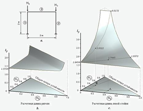
Fig.3

Figure 4 shows the analytical model of a 4-story 4-span frame. All rods of the same cross section. All floors are loaded with the same distributed load.

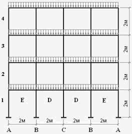
Fig.4

The graphs in Fig. 5 show the calculated curves of the coefficient of buckling length m for columns (A, B, C) and crossbars (D, E). The level of load with respect to the critical state is plotted on the abscissa scale. Numbers indicate floor numbers.

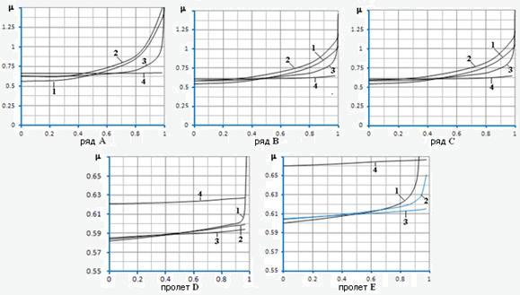
Fig.5

Table 1 gives the limit values of the coefficient m, corresponding to the critical state of the structure. Note that these limit values correspond exactly to the “standard” scheme of analysis, when load increases in all elements of the system simultaneously. As a consequence, for crossbars elements in which initially there were no effort, we obtain m=∞ (the effect of huge buckling lengths for lightly loaded elements is well known to the designers).

Table 1

 

Fig. 6a shows a truss reinforced at five points of the upper belt from its plane. Upper belt composed of I-beams СТО АС4М 20-93 16В2 (J_y=6.83∙10^-7m⁴, J_z=8.69∙10^-6m⁴). Lower belt - I-beam 12В2 (J_y=2.77∙10^-7m⁴, J_z=3.18∙10^-6m⁴). Braces and racks - square profile 60х6. Truss links - square 50х5.5. A vertical distributed load of 15,000 N/m is applied to the upper belt, which is 92% of the critical load (buckling occurs by lateral deflection from the truss plane).

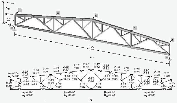
Fig.6

The calculated values of the coefficient of buckling length m: are shown next to each element of the truss in Fig. 6b: the upper values correspond to the bending of elements from the truss plane, the lower ones - in the truss plane. Fig. 7 shows the values of the coefficient of buckling length for elements of the same truss calculated according to the “standard” method.

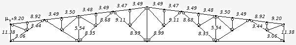
Fig.7

The standard method allows calculating the buckling lengths only for compressed elements and only when bending relative to one of the principal axes of the rod (in this case, when bending from the truss plane). As you can see, there is some correspondence between the values of the coefficient m_y for the elements of the upper belt between the attachment points of the support braces, calculated by both methods. All other elements are lightly loaded and for them the program produces unacceptable coefficient values m.

The algorithm described above was successfully implemented on the basis of the Selena software package [8]. The algorithm sequentially for each rod constructs a stiffness matrix of the truncated part of the system at the rod attachment points and then solves the eigenvalue problem for the tested rod under the found boundary conditions. The algorithm has shown its extreme effectiveness. Due to the fact that the eigenvalue problem splits into many small tasks, the algorithm works very quickly. So the analysis of a spatial frame system of 10x10 spans and 10 floors (1331 nodes, 3410 rods, tape width after renumbering 97 nodes) on a DELL 6400 computer (Intel Core 2 Duo T9550 processor, 2.66GHz) solved the problem for 14.4 seconds. (static - 5.7 sec.). It is important to note that within the framework of the proposed approach, there is no problem of “huge buckling lengths”. The buckling lengths can be calculated for both principal axes of the section independently from each other. The concept of “buckling length” can be quite naturally extended to unloaded, and even stretched elements. And, perhaps, most importantly, the formal approach to solving this problem allows us to almost completely automate the procedure for checking the local stability of bar sections.

Литература

1. Oppe M., Muller C.,Iles C., NCC: buckling length of columns; rigorous approach, London, Accsess Steel, 2005.

2. Webber A., Orr J.J., Shepherd P., Crothers K., The effective length of columns in multi-storey frames, Engineering Structures, 102 (2015),132-143.

3. СП 16.13330.2011, Стальные конструкции, СНиП II-23-81*, Москва, 2011.

4. AISC. AISC manual of steel construction. Load and resistance factor design. Chicago, AISC,2001.

5. Eurocode 3: Design of steel structures –Part 1-1: General rules and rules for buildings, EN 1993-1-1,2005.

6. Лейтес С.Д. Справочник по определению свободных длин элементов стальных конструкций, М.: Проектстальконструкция, 1967.

7. Бритвин Е.И., Тарнопольский А.А., К вопросу о проверке устойчивости стержневых конструкций, ж. Будiвницьтво Украiни, №1, 2006г. с.22-27.

8. Прочность, устойчивость, колебания. Универсальный программный комплекс для расчета конструкций на прочность SELENA. Сайт selenasys.com, -389 C.